Next: Comparison with a recent Up: Uncalibrated Stereo Correspondence Previous: Stereo matching by SVD

Some experimental results

 
     

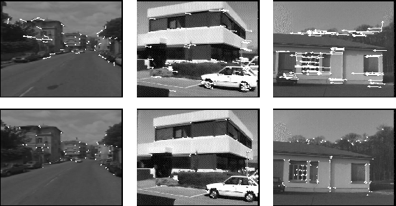
Figure 3: Some more test images pairs. Disparities are overlaid onto the top images and matching corners onto the bottom ones. Comments in Section 5 .

Several experiments have been performed on image pairs of various size and quality; some of the results are reported and discussed here.

The features were detected via the SUSAN corner detector [ 10 ]. In order for the correlation not to be too affected by noise, images were Gaussian smoothed. The key parameter in Equation ( 2 ) was set to 1/8 of the image width; more about this later in the section.

It is extremely important to point out that in order to illustrate the performance of the algorithm by itself , no further processing for filtering out bad matches has been applied. Most of the bad pairings that will be seen in the examples could have been simply eliminated by any commonly used technique, such as coherence of disparity.

Back to the first experiment, Figure 2 -left shows the disparities overlaid onto the first image and the corresponding corners on the second image (right); this method for presenting results will be used throughout. Being related by translation and rotation, this case involves non-uniform disparities but, as it can be seen, the results are extremely good and numerous 1:1 pairings have been found. It is encouraging to see how the method managed well to disentangle itself in areas where there is a large number of close-by features. Notably, a few good matches (about 10) have been missed out for some reasons such as low-correlation or simply because there were two or more equally competing alternatives.

Figure 3 -left presents the case of a poor quality road scene, with a remarkable expansion. It can be seen that although there are six mismatches, an overall good mapping was obtained. Note that near the focus of expansion the disparities cannot be very accurate working at pixel resolution.

Figure 3 -middle shows an image pair related mainly by translation. This case has some potential problems because of the clusters of features concentrated in the right-hand side of the image (e.g. the car wheel). The method has however performed exceedingly well, leaving just one grossly misjudged pairing.

Finally, Figure 3 -right presents another case that has prevalent translation. Here too there could be some difficulties due to the high displacement and the highly repetitive and identical features of the window and the tree leaves, respectively. Although 7 pairings are grossly wrong, the overwhelming majority is correct and would easily allow a robust next stage to operate.

The choice of the parameter , thanks to the better discriminating correspondence strength function, is fairly easy. The table in Figure 4 -right gives the number of mismatches (found by visual inspection) for the pairs in Figure 3 -middle and left with respect to changes in expressed as fraction of the image width.

It is clear that can vary within a relative large range without affecting performance too much. Having said this, in [ 8 ] it is suggested that the value of should reflect the average displacement of points; supportingly, our experiments also show that the best results are obtained when roughly matches the actual image displacement.