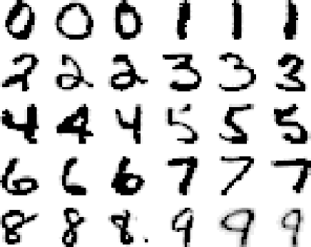
Figure 8: Some examples of the used
 character representations


In this section a number of character recognition experiments will be presented that illustrate the possibilities of some of the above discussed classifiers. In particular examples will be given that support the following observations:
Ā
Ā

Figure 8:
Some examples of the used character representations
These experiments are partially published before [16], [17]. They are
based on one of the NIST databases [18] from which we extracted 1250
samples for each of the ten handwritten numerals . In the raw data the characters are represented in binary
 images. We used the normalization software supplied with this dataset
and applied it for position, size, angle and line-width, resulting in
 gray value images. See figĀ
8
for some examples. The data was split into a fixed set of 250 characters
per class for training and 1000 characters per class for testing. All
experiments were run only once, using constant subsets of 5 until 250
characters per class.
Ā
Ā
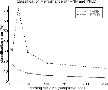
Figure 9:
Performance of the nearest rule (1-NN) and the pseudo-Fisher liner
discriminant
As a reference we computed first the (pseudo) Fisher's linear discriminant (PFLD) and the nearest neighbor rule (1-NN), see figĀ 9 . The PFLD shows the peaking behavior as discussed before, see figĀ 6 , for a sample size (1025) that is about the feature size (256). The nearest neighbor rule performs much better, indicating that nonlinear classifiers might be useful. In the following figures the 1-NN error curve is repeated as a reference. For the neural network experiments so called shared weights networks have been applied known as ``LeCun" (in our implementation 1361 neurons, 63660 connections and 9760 weights and biases), see [19], its extension ``LeNet" (4634, 94952, 6434), see [20] and the much smaller ``LeNotre" (394, 2210, 764), see [21]. Results are shown in figĀ 10 . For these sample sizes the 1-NN rule appears to perform better.
Ā
Ā
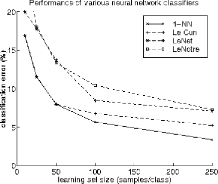
Figure 10:
Various neural networks compared with the nearest neighbor rule
The training of these large neural networks is computationally very heavy. Moreover, this also holds for the application of a neural network with many weights for the recognition of new objects. On both points SVC's might perform better. In our experiments, however, the training of a SVC using the by Vapnik proposed quadratic programming technique [5] took about 10 days on a Sun 200MHz Ultra-2 system for 250 objects per class. On the other side, the resulting performances are very promising, see figĀ 11 , where we show the results for classifiers up to degree 4.
Ā
Ā
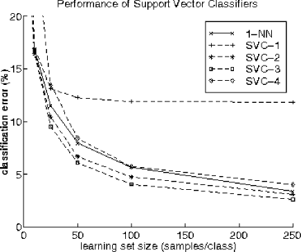
Figure 11:
Original support vector classifier compared with the nearest neighbor
rule
Ā
Ā

Figure 12:
Perceptron support vector classifier compared with nearest the neighbor
rule
Stimulated by the performance of Vapnik's support vector technique and
by Raudys' observations on the general possibilities of the perceptron
we developed a perceptron technique for optimizing the SVC. For
initialization the nearest mean classifier is used. As targets we set , in which
d
is the degree of the classifier and we trained for just 1000 epochs
using batch training with step size 0.001. The computational effort is
herewith reduced to about 10% compared with the quadratic programming
technique. Performances, shown in figĀ
12
, are for large sample sizes just slightly worse or even better.


Adrian F Clark