


Cartesian Differential Invariants describe the differential structure of an image independently of the chosen cartesian coordinate system. To construct these invariants we first extract the differential structure of the image. This is done using a scaled set of differential operators. The zeroth order operator, on which the rest of the operators are based, is the normalised isotropic Gaussian. The higher order operators are generated from derivatives of the Gaussian, allowing us to study the differential structure of the image up to any order using a set of discrete convolution filters.
The normalised Gaussian derivative Kernel is given by:
where is the scale and D is the number of dimensions.
The first order Kernels are:

The second order Kernels are:

and so on.
| Invariant | Order | Manifest Invariant Notation |

|
1 |

|

|
2 |

|

|
2 |
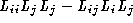
|

|
2 |

|

|
3 |
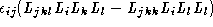
|

|
3 |
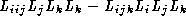
|

|
3 |
|

|
3 |

|
The set of all such filters completely determine the local image
structure. Notice that each filter has a single parameter,
, defining the scale of the filter. The response of the above filters
depends on the choice of cartesian coordinate frame. However, certain
combinations of filter response can be shown to be independent of the
choice of coordinate frame. These combinations are known as
Cartesian differential invariants
. TableĀ
1
shows a canonical set of eight two-dimensional polynomial invariants to
third order, expressed in tensorial manifest invariant index notation [
12
] (Appendix A).
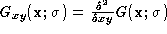
In order to ensure that the invariants are independent of the image's contrast, each tensor is divided by the L tensor (ie by intensity).
An obvious question to address, before basing any scheme on the use of differential quantities, is their reliability in the presence of noise. We have tested the invariants to see how they respond to noise. Typical results for a set of face images similar to those in Figures 2 and 5 are shown in FigureĀ 1 . We defined the error in response as:

where is the response of the invariant at point
 given an image with random gaussian noise of standard deviations
s
,
n
is the number of points sampled and
given an image with random gaussian noise of standard deviations
s
,
n
is the number of points sampled and is the standard deviation of all responses with no noise. The image
intensities were in the range 0 to 255.
is the standard deviation of all responses with no noise. The image
intensities were in the range 0 to 255.
Ā
Ā
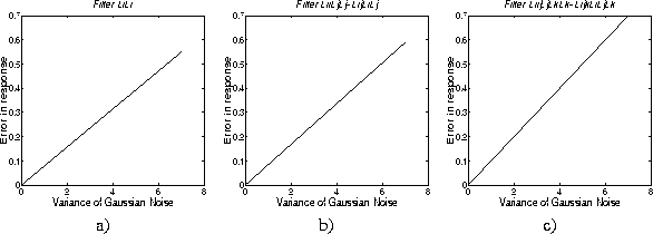
Figure 1:
Graphs showing the error in the response of (a)
, (b)
and (c)
at .
.
The results show that even for quite large noise amplitudes, the change in invariant values is small compared to the intrinsic variation across the image.
Kevin Walker
