Results

   
Figure: Original 200 by 200 pixel test images (viewing distance 55 cm)

Figures  5 , 7 and 8 show the results of some putative image resampling techniques applied to the test images, shown in Figure  4 . The first image contains black text (grey level 0) on a white background (grey level 255). Text rescaling via image resampling is interesting as character bitmaps are specially tuned to a particular resolution. The second image shows a simple landscape scene. The third image shows a human face and contains both over- and under-exposed regions. Each image in Figures  5 , 7 , and 8 has been contracted then expanded by a factor of four (not all of the methods allow expansion and contraction by anything other than integers). The methods that are compared here are:

1. Nearest neighbour interpolation   ;
2. Lowpass area m -sieving [ 1 ] to area ten with nearest neighbour resampling   - the sieve is a recent extension of mathematical morphology;
3. Lowpass recursive one-dimensional sieving [ 2 ] (vertical then horizontal) with nearest neighbour resampling   ;
4. Bilinear interpolation   ;
5. Polynomial spline interpolation [ 12 , 11 ] (here we use a first order B-spline)   ;
6. FFT interpolation [ 3 ]   ;
7. DCT interpolation [ 7 ]   ;
8. Group mean reduction followed by an edge enhanced interpolation [ 16 ]   .

The resampled images were shown to a human viewing panel consisting of 13 people. Each person was asked to score image quality on a ten point scale. The images from all resampling methods were presented simultaneously. An uncorrupted image was also included as a control. Each observers scores were then ranked (the control image was always judged the best so was removed from the rankings) and the mean and standard deviation of rank computed across all observers.

The viewing panel identified method 7 as the best image (mean rank of 1.5 in Table  1 ). Method 7 also has a low visual difference score, but not the lowest. In fact signal-to-error ratio correctly identifies the image our panel thought least distorted.

   
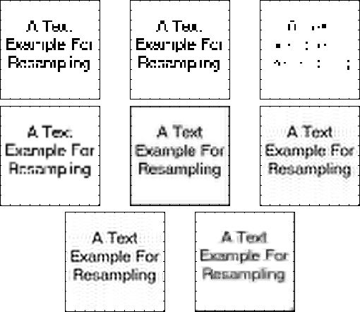
Figure: Text interpolated by, from left to right and top to bottom, methods 1 to 8 . The correct viewing distance is 55 cm.

   
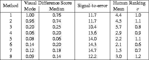
Table: Scores for the text image of Figure  5 .

Figure  5 shows the result of resampling the text image with these eight methods. Method 5 zero pads the image which gives a black border that we ignore here.

The visual difference score varies from pixel-to-pixel and its distribution may be complicated. For example in image  7 in Figure  5 the majority of pixels are in error, but the panel preferred this image to, say, image  1 in which the majority of pixels are uncorrupted. To some extent this effect is modelled by the foveal averaging, but clearly further investigation is necessary. Figure  6 shows histograms of the visual difference score after foveal averaging for three of the methods. The distributions are multimodal so a question arises. Do humans concentrate on the average error or some other distribution statistic? This question has not been resolved so we record the median and mode scores.

   
Figure: Histograms of Visual Difference Scores for Text images resampled by Methods  1 (left), 3 (centre) and 7 (right)

The vision model is adjusted so that one degree of visual arc is equivalent to 62 pixels (on our equipment this corresponds to a viewing distance of 1 m and puts the horizontal and vertical Nyquist frequencies at roughly rad deg ). Viewing Figure  5 at 55 cm gives the same effect. Visual scores produced by modelling the human vision system are dependent on viewing distance [ 10 ] so the results presented here are only valid for the distances stated. Some care is needed when interpreting Figure  5 and Table  1 as the Visual Difference Scores are not meant to model how well we recognise text: they are a measure of image quality. For this reason previously unseen images such as those in Figure  7 may give more consistent scores.

Table  2 gives the scores for Figure  7 . The panel of human observers chose methods  5 , and 8 as having the lowest errors. Methods  5 , and 8 also have low median and mode visual difference scores. Furthermore the median and mode are close together indicating a consistently low error over the whole image. Note that method 8 which is ranked highly by the panel and the visual difference scores has one of the lowest signal-to-error ratios, so in this case ranking by signal-to-error fails.

Figure  8 shows the face image. The scores are reported in Table  3 . Again the panel preferred methods  5 , and 8 , and these had consistently low visual difference scores.

   
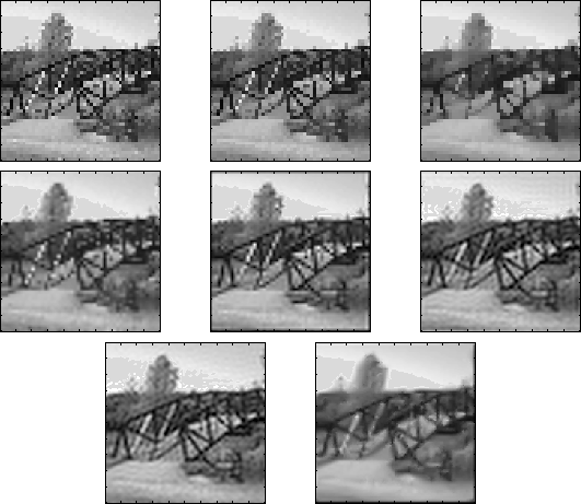
Figure: Bridge image interpolated by, from left to right and top to bottom, Methods 1 to 8 . The correct viewing distance is 55 cm.

   
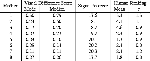
Table: Scores for the bridge images of Figure  7

   
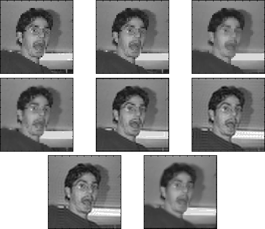
Figure: Face image interpolated by Methods 1 to 8 , reading from left to right. The correct viewing distance is 55 cm.

   
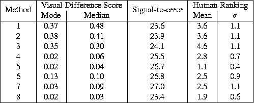
Table: Scores for the face images of Figure  8