 landmark points:


The point distribution model (PDM) is based upon the desired object being defined in terms of landmark points, positioned strategically on object features - often on the object boundary. By labelling such landmark points, a statistical approach can be used to extract the mean shape, and the modes of variation of a set of training examples.
Each training example (object outline) can be represented as a shape
vector containing landmark points:

Principal component analysis is then carried out on a set of
N
such training examples, so that each vector can be expressed in terms of a mean shape
 and a vector of weights
 signifying the influence of the modes of variation encapsulated within
the matrix of eigenvectors
 :
:

The landmark points are either hand-chosen for each image, which can be a laborious task when dealing with long image sequences, or alternatively by an automatic method for extracting the shape vectors [ 10 ].
Ā

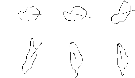
Figure 2:
Ā
Training examples; the arrows illustrate velocity, and the circles
represent the reference landmark on the principal axis
In the work reported here, a suitable segmentation process is used to
extract the shape of the flock of ducks, and thus the shape vectors from the noisy image sequences. Image sequences of a group of 6 ducks
moving around inside an arena 16m in diameter are taken using a fixed
camera mounted externally to the arena at a distance suitable for
observing the whole of the arena in the grey-scale image (see Figure
1
).
Incoming frames are subtracted from a pre-learned background image, and significant regions extracted by thresholding the difference with hysteresis; these regions are then subjected to morphological smoothing. Two separate regions are determined - one for the robot, and one for the flock as a whole. The outline of the flock region, together with the centres of mass of both regions, are stored and transformed from the image plane to world co-ordinates via a pre-determined transformation, based upon a known camera calibration. The above process allows automatic extraction of the position, velocity and shape parameters at up to 15 frames-per-second on widely available hardware.
The shape vector for each training example is calculated by taking uniformly spaced intervals along a B-spline approximation of the flock outline. In addition, a reference point is needed to order these points, taken to be the point on the principal axis nearest to the flock velocity vector. This may be a possible cause of error, but over a suitably large data set, the effects are reduced. Typical training examples for the PDM can be seen in Figure 2 .
The purpose of using principal component analysis is to achieve an
element of dimensional reduction in the model representation. For
example, if we use 20 control points on the flock outline, then there
will be 40 parameters in each shape vector , and thus 40 modes of variation. However, over 85% of the variation in
the training data is accounted for by the first 8 modes (see Table
1
), and thus we can reduce the dimensionality of the model, while
sacrificing only a small amount of accuracy, and eliminating small scale
variation probably attributable to noise.
| No. of modes used | 1 | 2 | 3 | 4 | 5 | 6 | 7 | 8 |
| Cumulative variation (%) | 34.1 | 59.8 | 67.2 | 73.9 | 77.9 | 80.7 | 83.2 | 85.7 |


N Sumpter