

Next:
5 Results
Up:
VOICI: Video Overview for
Previous:
Clustering by thresholding: a
We used the digital images of the Leiden 19th-Century Portrait Database
(LCPD)
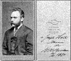
 as image database for our research. This database consists of images
taken from cards (scanned at 300 dpi), containing a picture of a
portrait from 19th-century on one side, and a studio logo or description
on the other. At the time, the LCPD image database contained 3014 images
which were obtained from 1507 cards.
Ā
Ā

Figure 2:
Example of a 19th-century LCPD image
Several methods have been developed for computing a similarity measure
of images. The methods differ in pixel domains, feature vectors and
metrics. The pixel domains can be categorized in the following groups:
-
-
-
intensity :
A method based on the intensity pixel values of images
-
-
-
gradient :
This method uses the derivatives of the intensity image.
-
-
-
binary :
the gradient values are thresholded to obtain a bi-level image.
Within each domain, we can choose feature vectors that represent the
image information. We shall mention a few of those methods (the
performance of which can be inspected using our LCPD WWW demo) here:
-
Horizontal/Vertical projections [
4
]
-
Pixel by pixel
-
Trigrams [
5
]
-
Local Binary Pattern (LBP) [
7
]
Given a set of feature vectors similarity can be quantified using
distance measures like the L1- or L2-norm. We used a method that was
based on the feature vector that describes the statistical distribution
of 2D tri-grams of 3x3 black & white pixels. We shall briefly explain
the trigram method in the following section; other methods are explained
in [
8
].
In [
5
] 2D pixel trigrams are introduced. Trigrams are based on statistics of
binary 3x3 texels in a thresholded gradient space. To create a gradient
space, we used the Sobel gradient. Once we threshold the gradient image
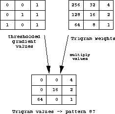
into binary gradient images, we can use trigrams. A trigram is a 3x3
texel of 1 bit values that form a 9 bit long string, 9 values of
different powers of 2 (1,2,4,...,256). The idea is to create a histogram
of 3x3 patterns, where there are a possible binary 3x3 patterns. Every possible 3x3 region in the binary gradient
image is multiplied with the trigram weights to obtain an index into our
histogram. The histogram value at this index is then raised by one. When
all possible 3x3 texels have been visited, a frequency histogram of the
binary image, with respect to all possible 3x3 binary patterns, is
obtained. These feature vectors are normalized before used for matching.
See figure
3
for an example of a computation that results in an index into a
histogram.
Ā
Ā

Figure 3:
Example of trigram pattern number calculation
Our histogram can be seen as a feature vector of length 512 of the
image. We can compute all the feature vectors of our images in the
database, and use the vectors for similarity matching. Similarity
matching is done by summing the absolute differences of the
corresponding feature vector elements for a pair of images (L1-norm).
Because this feature vector is rather large (512 different patterns as
mentioned before) and contains a relatively large fraction of noise
contributions, a bandpass filter is used to suppress all but 75 patterns
during the comparison. The resulting distances are stored in a full
distance matrix which is used to generate an overview of the Leiden
19th-Century Portrait Database. In [
6
] the effectiveness of Trigram feature vectors for image comparison is
compared against the performance of projections, Local Binary Patterns
and Virage Datablade.


Next:
5 Results
Up:
VOICI: Video Overview for
Previous:
Clustering by thresholding: a
Dr. D.P. Huijsmans
Tue Jun 24 15:22:02 MDT 1997
 as image database for our research. This database consists of images
taken from cards (scanned at 300 dpi), containing a picture of a
portrait from 19th-century on one side, and a studio logo or description
on the other. At the time, the LCPD image database contained 3014 images
which were obtained from 1507 cards.


 binary 3x3 patterns. Every possible 3x3 region in the binary gradient
image is multiplied with the trigram weights to obtain an index into our
histogram. The histogram value at this index is then raised by one. When
all possible 3x3 texels have been visited, a frequency histogram of the
binary image, with respect to all possible 3x3 binary patterns, is
obtained. These feature vectors are normalized before used for matching.
See figure